
Back to Contents
Business Software I – Microsoft Excel Spreadsheet Other Commands
Apart from calculations, other powerful and useful features are sorting, filters and generating graphs / reports. There is a demo that can be used from Microsoft which is at this URL
Saving File Names (so that original data is not touched and mucked up)
The following data is something created for this exercise similar to previous exercises but just a few more details of customers added to make it realistic.
You should really work with a different version of the file ie a copy of that file so that you have the original data entered remains intact in case you made some errors and data got mucked up. Filtering can muck up data if not used correctly.
To save a copy of the same file to work with in terms of Filtering or Reporting, use the “Save As” not just “Save”
ie File –> Save As to a different filename eg
1999_04_14_sydney_hailstorm_customer_details_excel_spreadsheet_filtered.xls
The original data was in this file
1999_04_14_sydney_hailstorm_customer_details_excel_spreadsheet_custom.xls
Sorting and Filters
Sorting and filters are used to extrapolate or extract useful data for management purposes. You spend time during the busy part of the day quoting and data is entered. During the evening hours or less busy periods, your management takes over, You may wish to find out who has not paid their excess, who has not booked in to repaired their cars yet, which parts have not arrived, what pricing on average is being repaired, which workers are producing the most cars – the list is endless.
Sorting is a quick command to sort in alphabetical and numerical order – increasing (ascending – smallest to largest) or decreasing (descending – largest to smallest).
| Automatically Sorts columns in Alphabetical Order | |
| Automatically Sorts columns in reverse Alphabetical Order |
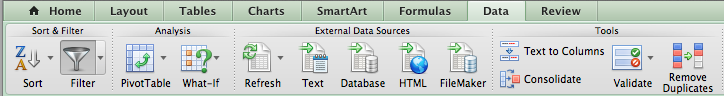
In the data toolbar (once you select Data between Formulas and Review), you will see a Sort button first followed by Filter button. These are described in this section.
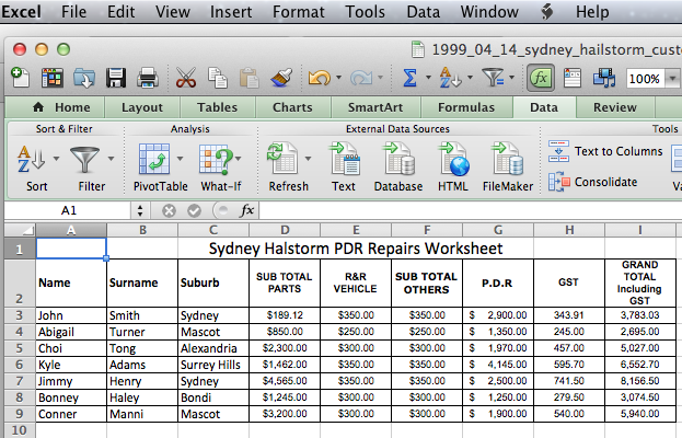
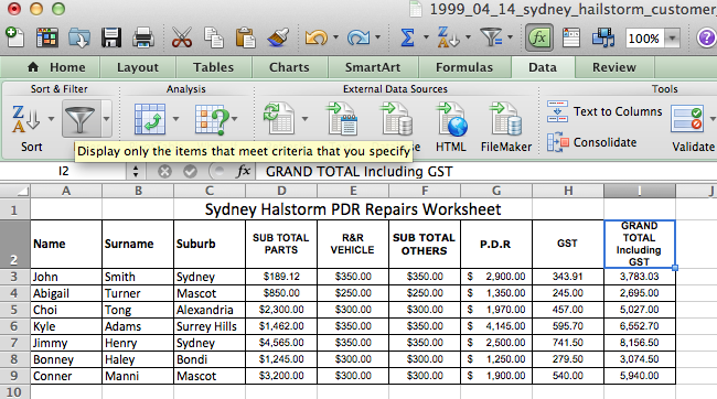
Consider the following table of data which consists of names, the suburb and pricing. We will use this simple table to show how data can be sorted and filtered.
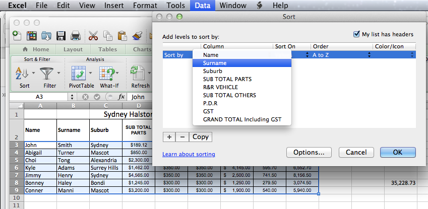
If we wish to sort in alphabetical order by “surname” basically column B, go to data in the menu Data, choose “Surname” to sort by, leave Order as A to Z press ok. Alternatively you can press the Data button on the toolbar and then ![]()
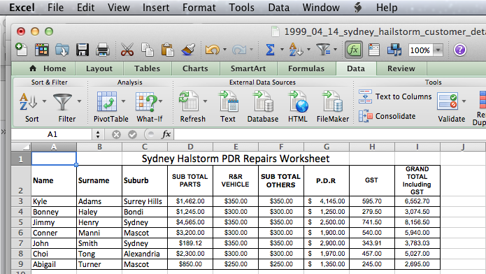
You should see the following result, all information including all rows of data has been sorted accordingly and has remained together which is important in terms of keeping the integrity of the data
You can easily sort this data if you wish based on the Grand Total “Column I” .
This time we will set up filters first. Filters are a more custom way of sorting in many different ways. So to order the least expensive to the most expensive jobs for example or to find the jobs that cost more than $5000 can be found. You quickly see how powerful it is in extracting the wanted data quickly – a type of reporting for your company.
To sort the data from least expensive to most expensive, ascending order,
–> CLick Data (on the toolbar between Formulas and Review)
–> Move your arrow or cursor as it is called to one of the headings eg Grand Total Columns (remember we want to filter the information from those columns.
–> Then Filter button (darker shaded when pressed here) which is highlighted next to the sort button
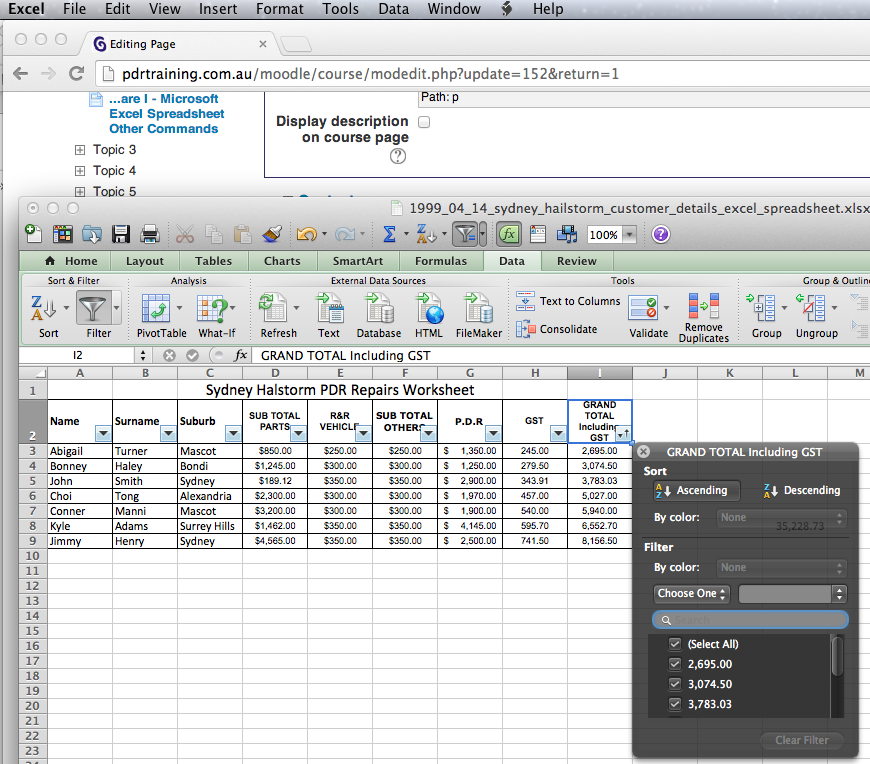
The columns will show filter (drop down arrow) buttons as follows near each heading Name, Surname, etc. These have become the filters for those columns.

Now this is very powerful as you can now order or filter any column by pressing the arrows next to each column heading – lets try pressing “Grand Total” down arrow. A pop-up menu should come up with options with the heading of the filter you chose – in this case “Grand Total including GST“. These options are the many types of filter conditions you can use!
Try pressing “Ascending” in this pop-up menu.
Now since this column contains only numbers, it will try and sort by letters alphabetically first, and since there are no letters, it will order the numbers. The numbers are now ordered. You can close the Filter pop-up and it will remain in order!
Notice that all the other information in the rows related to the job including the customer details have moved in that order based on this filter of Ascending. The data has to stick together otherwise it will not be useful.
How about trying to do the same but find the Grand Total in Descending order. Instead of Ascending choose Descending in the pop-up menu.
If you are not going to use Filters, you can switch it off by pressing it again and all the Filter down arrows will be gone and the data should be there.
Further Data Filtering
Now, this next section will show you how powerful filtering really is! Why do we use filters? When you have hundreds of customers’ details entered on the system, trying to find the one you wanted or just getting an idea of where things stand within the business is why you may need to narrow down your data to find specific information. For instance, finding the most expensive jobs, the jobs that were between a certain cost range, repeat customers, grouping customers from specific suburbs, grouping by insurance companies and so on. Filters can narrow this information in a few clicks.
Exercise 1
What if we wish to find all jobs in the Sydney hailstorm data that were great than $5000 Grant Total? Easy. If the Data, Grand Total and Filter Column are still highlighted as above, ignore the following. If you had switched it off, then just do it again
–> CLick Data (on the toolbar between Formulas and Review)
–> Move your arrow or cursor as it is called to one of the headings eg Grand Total Columns (remember we want to filter the information from those columns.
–> Then Filter button (darker shaded when pressed here) which is highlighted next to the sort button
(Remember the Filter is witched on when those down arrows are next the headings).
Now click the down arrow next to Grand Total again since we are going to filter our data based on the total prices above $5000.
–> Below the By color, I there is a Choose One filter button, click that and look how many options

In the following example, you can see after the pop-up came in view and I chose in the Choose One section “Greater Than”
I typed in next to the Greater Than 5000 ( no need to put in $). You will notice that instantly, the data that have only Grant Totals greater than $5000 pricing will be showing – others are hidden. Don’t panic, they are not lost – just hidden from view.

This technique allows managers to filter data they wish to use and browse through them as browsing through certain information may be useful for planning purposes.
Please note, do not save the data in this fashion with filters. Leave the original data alone and undisturbed in case you make a mistake with the data and save this file as a different filename.
Exercise 2
Now what if we wish to filter our customers by suburbs to group all customers within those suburbs together.
